How to Reduce E-Commerce Return Costs: Dynamic Routing Algorithms vs Static Logistics Rules

1. Introduction to the Problem and Target Audience

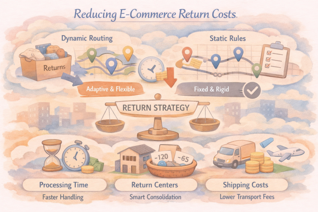
The modern e-commerce industry faces a massive challenge that destroys profit margins: reverse logistics. When a customer returns an item, the company must decide what to do with it. Historically, businesses have treated this as a simple transportation task. However, the volume of returns has grown to a point where moving boxes without thinking causes severe financial damage. This document is a comprehensive guide designed for Chief Financial Officers, Supply Chain Directors, Data Engineers, and E-commerce Product Managers who need to stop losing money on returned goods.

The core problem is that traditional companies use static rules to manage returns. These rules do not consider real-time data, changing shipping prices, or the actual value of the specific item at that exact moment. To solve this, businesses must transition from rigid rules to a dynamic cost graph algorithm. This means calculating the most profitable route for every single returned item in real-time, right at the moment the customer hands it back.

Target Audience	Core Business Problem	Primary Technical Challenge
Supply Chain Directors	High transportation costs for returning low-value items.	Inability to change routing rules quickly when transport rates increase.
Chief Financial Officers	Profit margins are destroyed by hidden processing and warehouse costs.	Lack of clear visibility into the exact cost per returned item.
Data Engineers	Static decision systems cannot handle complex, real-time variables.	Need to build high-throughput backend services without database bottlenecks.
Store Managers	Physical stores become filled with returned items that nobody wants to buy locally.	Frontend interfaces for staff are too slow and confusing to use during busy hours.

2. Real-World Case Studies and Analysis

To understand why static rules fail and why algorithmic routing is necessary, we must look at how things happen in reality. The following case studies demonstrate the conflict between basic logistics rules and the actual financial reality of e-commerce.

Case Study A: The Fast Fashion Apparel Crisis

A large online clothing retailer uses a static rule: “All returned winter jackets must be sent back to the central warehouse for quality control.” A customer in a distant region returns a jacket that costs 30 euros. The static rule forces the local collection point to ship the jacket across the country.

Fact / Argument Category	Traditional Static Rule Approach	Reality Conflict	Algorithmic Solution
Transportation Fact	The system automatically generates a shipping label to the central hub.	Shipping from a distant region costs 12 euros.	The system checks the API for transport costs before making a decision.
Processing Fact	The item is processed at the central warehouse by specialized staff.	Quality control, repacking, and restocking cost an additional 8 euros in labor.	The algorithm calculates that processing costs are too high for this item’s value.
Market Value Fact	The item is placed back on the website at full price.	The winter season is ending; the jacket will only sell with a 50 percent discount (15 euros).	The system predicts the seasonal markdown immediately.
Final Financial Argument	The business believes it saved the item for resale.	Total cost is 20 euros. Resale value is 15 euros. The company loses 5 euros on a successful sale.	The algorithm orders the local store to mark down the item to 10 euros locally, saving transport costs and generating a small profit.

Case Study B: High-Value Consumer Electronics

An electronics store sells a smart vacuum cleaner for 400 euros. The customer returns it saying it does not work. The static rule says: “Keep electronics in the local store for quick resale to save transport costs.”

Fact / Argument Category	Traditional Static Rule Approach	Reality Conflict	Algorithmic Solution
Condition Assessment Fact	Local store staff quickly look at the box and put it on the discount shelf.	Local staff lack the tools to test complex electronics properly.	The algorithm flags high-value electronics with mechanical error codes for central diagnostics.
Financial Risk Argument	The store saves 15 euros on shipping.	The next customer buys the broken vacuum, gets angry, and leaves a terrible review, demanding a full refund.	The algorithm accepts the 15 euro transport cost to save a 400 euro asset from total destruction.
Inventory Data Fact	The local store system shows one used vacuum in stock.	Nobody in that specific local neighborhood wants a used premium smart vacuum.	The algorithm analyzes regional demand and routes the item to a region with high search traffic for this model.
Core Conclusion	Static rules try to save small amounts of money on shipping.	Saving on shipping for high-value items often results in massive brand and product losses.	Dynamic routing spends money on shipping only when the expected recovered value justifies the cost.

Case Study C: Seasonal Home Goods

A company sells large garden furniture. Returns happen frequently because the colors do not match the customer’s garden. Static rule: “Return all large items to the central hub.”

Fact / Argument Category	Traditional Static Rule Approach	Reality Conflict	Algorithmic Solution
Capital Fact	Furniture takes up massive space in transport trucks.	Transporting a returned garden sofa costs 80 euros due to its physical dimensions.	The algorithm calculates volume-to-value ratio in real-time.
Time Constraint Argument	The item spends 14 days in the reverse supply chain.	By the time it reaches the central warehouse, the summer season is over.	The system identifies the time delay and realizes the item will sit in storage for 9 months.
Warehouse Storage Fact	The item is stored until next spring.	Storage costs for large items destroy any remaining profit margin over 9 months.	The algorithm calculates storage depreciation and suggests immediate local disposal or extreme local discount.

3. The Algorithm: Design, Purpose, and Technical Implementation

The goal of the dynamic cost graph algorithm is to calculate the single most profitable action for every returned item at the exact moment it is scanned by the receiving worker. We move away from “IF-THEN” statements and start using mathematical expected value.

The Mathematical Logic (Standard Text Representation)

Because we cannot use complex formatting, the logic is represented in plain text formulas. The algorithm must calculate the Expected Profit for every possible destination (Node A: Central Warehouse, Node B: Local Discount, Node C: Recycling).

Formula 1: Expected Recovery Value equals the Base Retail Price multiplied by the Probability of Sale minus the Expected Discount.

Formula 2: Total Route Cost equals Transport Cost plus Warehouse Processing Cost plus Expected Storage Depreciation.

Formula 3: Final Node Score equals Expected Recovery Value minus Total Route Cost.

The algorithm runs these calculations for all available routes. It then selects the route with the highest Final Node Score. If all scores are negative, the algorithm immediately issues an instruction to recycle or destroy the item locally, preventing any further money from being wasted on a lost cause.

Algorithm Parameter	Data Source	Purpose in the Calculation
Base Retail Price	Central Enterprise Resource Planning system (ERP).	Establishes the maximum possible money we can get back.
Probability of Sale	Historical sales data and current regional search trends.	Lowers the expected value if the item is unpopular or out of season.
Transport Cost	Real-time API calls to courier services or internal fleet databases.	Calculates the exact penalty for moving the item from point A to point B.
Processing Cost	Fixed labor costs per minute tracked in the warehouse management system.	Adds the human labor cost required to check, clean, and repack the item.
Storage Depreciation	Daily cost of shelf space multiplied by expected days until sale.	Prevents sending large, cheap items to expensive central warehouses.

Technical Architecture and Data Engineering

To make this work in reality, the backend must be incredibly fast. When a worker scans a barcode, they cannot wait 10 seconds for the system to think. The decision must appear in under one second.

The architecture relies on a highly concurrent backend, often built in languages like Go, capable of processing hundreds of thousands of requests per second during peak holiday return seasons. The system receives the scanned item ID and instantly creates multiple independent concurrent requests to fetch the ERP data, the transport API rates, and the historical data.

We must also monitor the cost of the algorithm itself. Running complex real-time queries can become expensive in cloud environments. Therefore, all transaction logs and calculation paths are streamed into a data warehouse like BigQuery. Here, data engineers deploy monitoring scripts to track the exact gigabytes processed per day, calculating the cloud cost per individual user and per data table. This ensures the routing system does not cost more to run than the money it saves.

For the frontend used by warehouse staff, we must track their interactions to ensure the interface is not confusing. By configuring custom event tracking in the dataLayer, we can monitor how long it takes a worker to process an algorithm’s instruction. If an item cannot be identified, the system must not use generic error labels; it should use specific missing parameter notations, such as labeling unattributed data strictly as ‘not_add’ rather than a vague ‘(not set)’. This strict data hygiene allows analysts to debug bottlenecks using synthetic browser testing.

Technical Component	Implementation Fact	Business Argument
Backend Processing	High-throughput Go service handling concurrent API requests.	Ensures the warehouse worker receives a routing decision in under 800 milliseconds, preventing queues.
Cloud Cost Monitoring	BigQuery automated dashboards tracking data volume.	Prevents runaway cloud costs by providing clear visibility into cost per table and cost per user query.
Frontend Tracking	DataLayer variables routing custom events to analytics platforms.	Allows product managers to A/B test the worker interface to find the most efficient button layouts.
Data Hygiene	Using strict missing data labels like ‘not_add’ instead of defaults.	Eliminates confusion during database analysis when tracking why an item failed to route properly.
System Reliability	Automated synthetic testing of the web platform and API endpoints.	Detects script-loading delays before they cause a massive disruption in the physical warehouse.

4. Algorithm Goals, Expectations, and Final Results

When a business implements this dynamic cost graph, the expectations must be clearly defined. The goal is not to eliminate returns—that is impossible in e-commerce. The goal is to maximize the residual value of the returned asset and eliminate empty, unprofitable logistics movements.

Implementing the Process

When you first turn on the algorithm, it will conflict with human intuition. A warehouse manager might see a perfectly good pair of shoes being sent to the trash compactor and think the system is broken. However, the system knows that shipping those shoes costs 10 euros, storing them costs 5 euros, and they will eventually sell for 12 euros. Throwing them away is mathematically the most profitable action.

To implement this smoothly, businesses must start with a shadow deployment. The algorithm runs in the background and logs what it would have done, while the static rules continue to operate the physical warehouse. Data engineers then compare the costs of the static rules versus the theoretical costs of the algorithm over a two-week period. Once the financial argument is proven, the business switches the routing logic to the live algorithm.

Implementation Phase	Expected Fact	Argument for this Approach
Phase 1: Data Integration	It will take significant time to clean ERP data (weight, dimensions).	Without accurate physical dimensions, transport cost APIs will return wildly incorrect prices, ruining the graph.
Phase 2: Shadow Mode	The algorithm will suggest destroying up to 15 percent of cheap returns.	Proves to management that forced restocking of cheap items is currently generating hidden financial losses.
Phase 3: Live UI Testing	Workers will initially make mistakes following the dynamic prompts.	Using custom dataLayer tracking on the frontend allows rapid iteration of the UI until worker error drops to zero.
Phase 4: Full Automation	Logistics providers will notice a drop in return transport volume.	The algorithm naturally filters out the “dead weight” items, keeping them localized and freeing up truck capacity.

Final Real-World Results and Trade-offs

After full implementation, companies typically see a massive shift in their logistics spending. The number of items traveling back to the central warehouse drops significantly. Instead, local markdown sales increase, and the volume of items liquidated locally goes up.

However, we must be honest about the weaknesses and trade-offs of this system. It is highly dependent on network stability. If the central data warehouse experiences an outage, the entire reverse logistics chain stops. The system also requires continuous maintenance of transport pricing models. If a courier changes their pricing structure and the API is not updated, the algorithm will make catastrophic financial decisions at scale.

Business Metric	Static Rules Result	Dynamic Algorithm Result	Strategic Argument
Average Transport Spend per Return	Consistently high, regardless of item value.	Drops by 30 to 40 percent.	Money is only spent moving items that have a guaranteed high resale margin.
Time to Resale	14 to 21 days due to central processing bottlenecks.	1 to 3 days for locally routed items.	Keeping items local allows them to be sold before seasonal demand disappears completely.
Cloud Infrastructure Costs	Very low, as rules are simple IF-THEN scripts.	High, requiring real-time calculations and BigQuery monitoring.	The business trades cheap logistics software for expensive cloud computing, but the net savings are massive.
Worker Training Time	Fast. “Put everything in the red box.”	Slower. Workers must follow specific screen instructions for every item.	The complexity is moved from the manager’s office to the worker’s screen, requiring better UI design and clear instructions.
Environmental Impact (ESG)	High carbon emissions from transporting garbage across the country.	Lower emissions due to localized processing, but higher local waste.	While local recycling increases, the massive reduction in unnecessary truck miles significantly lowers the carbon footprint.

In conclusion, managing a 30 percent return rate in modern e-commerce requires treating every returned item as a unique financial equation. Static rules are a relic of a slower era. By implementing a dynamic cost graph, utilizing high-speed Go backends, strictly monitoring cloud database costs, and maintaining clean frontend tracking parameters, a business can transform reverse logistics from a massive financial bleed into a tightly controlled, optimized recovery operation. The transition requires significant engineering effort, but the protection of the profit margin makes it an absolute necessity.