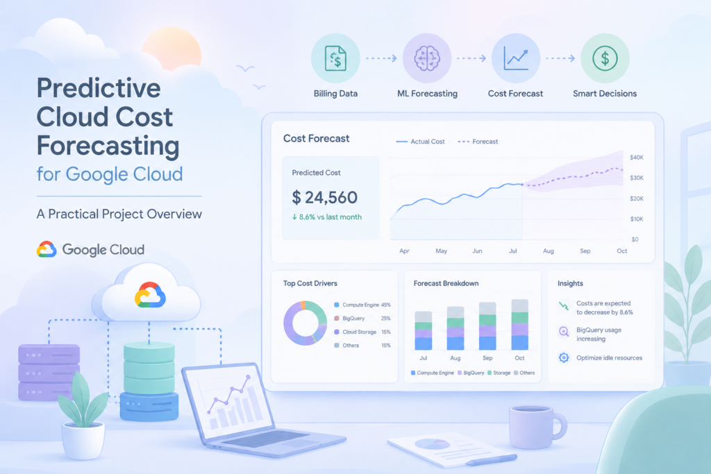
Predictive Cloud Cost Forecasting for Google Cloud: a Practical Project Overview

Cloud cost unpredictability is a persistent business problem. For organizations that rely on Google Cloud Platform, the dominant cost drivers are storage, query scan volume (especially BigQuery), streaming ingest, and egress. A predictive analytics system that forecasts these drivers and translates them into monetary estimates becomes a strategic tool: it enables proactive FinOps, targeted optimization, and reliable budgeting. This article describes a project blueprint for building such a system: the business objective, the modular decomposition, the modeling approaches and algorithms, the architecture and components, the evaluation metrics, and the principal risks with concrete mitigations. The description is technology‑agnostic in spirit but assumes implementation using F# and the .NET ecosystem for data processing, modeling, and service orchestration.

Business problem and value proposition The core business problem is twofold: first, cloud spend is volatile and often driven by a small number of heavy queries, misconfigured pipelines, or unexpected egress; second, teams lack timely, actionable forecasts that map technical usage to financial impact. The predictive system must answer three operational questions: what will we consume tomorrow (or next hour) across storage, scanned bytes, streaming ingest and egress; what is the expected dollar cost under current pricing; and which resources or jobs are the most likely contributors to forecast error or spikes. Value flows from early detection of cost drift, prioritized optimization recommendations (e.g., partitioning, query rewrite, materialized views), and improved budgeting accuracy.

Modular decomposition A robust implementation separates concerns into clear modules. Each module has a focused responsibility and well‑defined inputs and outputs.

1. Data Ingestion and Normalization Collect billing exports, BigQuery job logs, INFORMATION_SCHEMA query metadata, streaming ingest metrics, and storage usage snapshots. Normalize timestamps, unify identifiers (project, dataset, job owner), and tag records with business metadata (team, environment, cost center). A synthetic data generator is useful for development and testing.
2. Aggregation and Feature Store Aggregate raw events into time buckets (hourly and daily) and compute rolling statistics. The feature store holds time series per metric and derived features: rolling means, variances, counts of heavy queries, partitioning ratios, number of dashboards refreshed, and calendar features (weekday, hour, holiday flags).
3. Modeling and Forecast Engine Implement a layered modeling strategy: lightweight online models for immediate forecasts and heavier batch models for improved accuracy. The engine exposes a uniform inference API and supports model selection and ensembling.
4. Cost Mapping and Business Translation Apply pricing rules to predicted volumes to produce monetary forecasts. Pricing logic must be parameterized to reflect tiered rates, discounts, committed use, and regional differences.
5. Anomaly Detection and Alerting Monitor residuals between predictions and observations. Implement statistical detectors (CUSUM, EWMA on residuals) to flag unexpected spikes and trigger alerts with contextual diagnostics.
6. Explainability and Prioritization For each forecasted spike or high‑cost driver, compute contribution scores that attribute predicted cost to datasets, jobs, or teams. This enables prioritized remediation.
7. API, Dashboard and Reporting Expose forecasts, historical comparisons, and alerts via a REST API and a dashboard. Reports should include confidence intervals, top contributors, and suggested actions.

Modeling approaches and algorithms A pragmatic system combines simple, robust time‑series methods with multivariate regression and optional machine learning ensembles. The goal is reliable, interpretable forecasts that can run online and be retrained periodically.

Baseline online models

• Exponentially Weighted Moving Average (EWMA): fast, low memory, suitable for short‑term smoothing and online updates.
• Holt‑Winters (additive or multiplicative): captures level, trend and seasonality for metrics with clear periodic patterns.

Statistical time series

• ARIMA / SARIMA: for series with autoregressive and moving average structure; useful when seasonality and differencing are required. Implementations can be adapted from numerical libraries or wrapped from existing .NET packages.
• State‑space models: Kalman filter variants for handling missing data and irregular sampling.

Multivariate and hybrid models

• Online linear regression with stochastic gradient updates: incorporate exogenous features such as number of dashboards, scheduled job counts, or recent heavy query flags.
• Regularized regression (Ridge/Lasso) for feature selection and stability.
• Ensembles: weighted combination of statistical forecasts and regression outputs to capture both temporal dynamics and external drivers.

Anomaly detection and residual analysis

• Residual z‑scores and moving variance thresholds.
• CUSUM and EWMA on residuals to detect sustained deviations.
• Rule‑based heuristics for known operational patterns (e.g., end‑of‑month reporting spikes).

Explainability and attribution

• Shapley‑inspired contribution approximations for regression models.
• Simple proportional attribution for time series: allocate predicted increase to datasets or jobs by recent contribution share.

Architecture and components Design the system as a pipeline of composable services with clear data contracts.

Data layer

• Sources: Cloud Billing export, BigQuery job logs, streaming metrics, storage snapshots.
• Storage: a time series table in BigQuery or a lightweight time series DB for fast reads; raw exports retained in object storage.

Processing layer

• Batch ETL: scheduled jobs to compute daily aggregates and retrain batch models.
• Stream/online layer: incremental aggregators and online model updaters for near‑real‑time forecasts.

Modeling layer

• Forecast service: exposes endpoints for inference, accepts time window and granularity, returns point forecasts and confidence intervals.
• Training service: orchestrates batch retraining, backtesting and model selection.

Application layer

• API: REST endpoints for forecasts, anomalies, and contributor lists.
• Dashboard: visualization of forecasts, historicals, and top contributors.
• Alerting: integrates with Slack/email and includes diagnostic payloads.

Operational layer

• Configuration: pricing rules, thresholds, and team mappings stored in a versioned configuration store.
• Observability: metrics for model performance (MAE, MAPE), pipeline health, and alert volumes.
• Access control: role‑based access to forecasts and cost drivers.

Evaluation metrics Measure both statistical accuracy and business impact.

Forecast accuracy

• Mean Absolute Error (MAE) and Root Mean Squared Error (RMSE) per metric and per time horizon.
• Mean Absolute Percentage Error (MAPE) for relative error assessment.
• Coverage of prediction intervals.

Business KPIs

• Monthly forecast variance: difference between predicted and actual spend.
• Frequency and lead time of detected cost spikes.
• Reduction in surprise spend after interventions (tracked over time).

Operational metrics

• Throughput and latency of the inference API.
• Data freshness and ETL success rate.
• False positive rate of anomaly alerts.

Risks and recommendations Data completeness and tagging risk Incomplete or poorly tagged job metadata undermines attribution and multivariate modeling. Mitigation: enforce tagging standards, instrument heavy jobs, and backfill metadata where possible.

Tail events and ad‑hoc investigations Large, infrequent ad‑hoc queries can dominate costs and are hard to predict. Mitigation: model tail risk explicitly (quantile forecasts), maintain a catalog of known heavy jobs, and implement quota/approval gates.

Model drift and seasonality shifts Workload patterns change with product launches or organizational events. Mitigation: continuous backtesting, automated retraining triggers based on drift detection, and human review for model updates.

Pricing complexity and contractual nuances Discounts, committed use discounts, and tiered pricing complicate cost mapping. Mitigation: parameterize pricing logic, validate forecasts against billing exports, and surface assumptions in reports.

Operationalizing recommendations A predictive forecast is only valuable if it leads to action. Integrate the system with FinOps workflows: surface prioritized optimization candidates, provide reproducible diagnostics for engineers, and track remediation outcomes. Maintain a feedback loop where post‑action outcomes feed model retraining and attribution accuracy improves over time.

Conclusion A predictive cloud cost forecasting system for Google Cloud is a high‑leverage FinOps capability. By decomposing the problem into ingestion, aggregation, modeling, cost mapping, anomaly detection and explainability modules, teams can build a pragmatic, interpretable solution. Combining lightweight online models with batch statistical methods and multivariate regressions yields robust forecasts and actionable insights. The result is not only better budgeting but a disciplined, data‑driven approach to reducing cloud waste and aligning engineering behavior with financial outcomes.

We build, migrate, and optimize cloud data pipelines on Google Cloud Platform. From BigQuery query optimization to custom ingestion architectures, explore our Data Engineering on GCP services.