How BigQuery Clustering Works: Inside the Capacitor Storage Format

1. The Wrong Mental Model: Sorting vs. Intelligent Organization

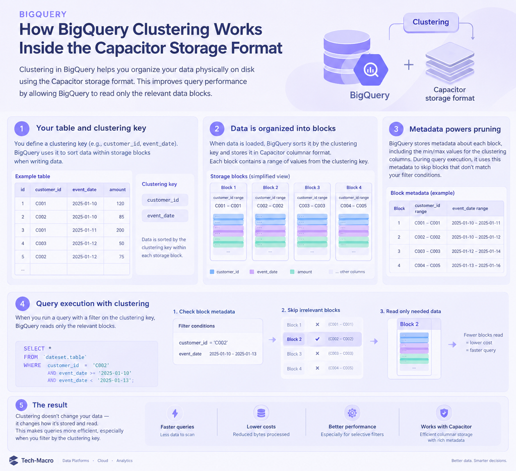
When engineering teams design analytical data platforms, they often carry over habits from traditional relational database management systems (RDBMS) like PostgreSQL or MySQL. Ask an engineer what clustering does in BigQuery, and the most common answer is: “It sorts the data.”

This is a dangerous oversimplification. In traditional OLTP (Online Transaction Processing) databases, indexes (like B-trees) rely on perfect sequential order. Finding a specific row is fast because the database traverses a tree in $O(\log N)$ time, pulling exact pages from the disk.

BigQuery does not promise perfect order. In fact, attempting to maintain perfect global sorting on a petabyte-scale distributed system would require constant rewriting of files, leading to catastrophic I/O bottlenecks. Instead, BigQuery promises intelligent organization.

Analytical databases care very little about finding one specific row. You do not analyze a massive web analytics dataset to find a single user’s click; you process the entire volume to find systemic trends and funnel drops. The primary goal of an analytical storage engine is not exact positioning, but efficient elimination of unnecessary work.

2. Under the Hood: Storage Blocks and The Capacitor Format

To understand clustering, we must discard the “giant spreadsheet” mental model. BigQuery does not store rows. It stores data in a proprietary columnar format called Capacitor, which is compressed and divided into distributed storage blocks.

When you insert data into a clustered table, BigQuery does not lock the table to sort billions of rows. Instead, as data is written to the underlying Colossus file system, BigQuery analyzes the clustered columns and attempts to group similar values into the same storage blocks.

The Mechanics of Block Elimination

When you execute a query, the Dremel execution engine reads the metadata of these blocks. If you filter by a clustered column (for example, event_name or traffic_channel), the engine performs a Predicate Pushdown. It checks the metadata (min/max values, dictionary encoding) of each block. If a block’s metadata proves it does not contain the requested value, BigQuery completely skips it.

• Processors are not computing faster; they are simply avoiding work.
• Without Clustering (Full Scan): I/O Cost is $O(N)$, where $N$ is the total data volume.
• With Clustering (Block Elimination): I/O Cost approaches $O(K)$, where $K$ is the volume of blocks containing the target data ($K \ll N$).

In BigQuery’s on-demand pricing model ($6.25 per TB scanned), reading a skipped block costs exactly $0.00.

3. Architecture Comparison: BigQuery vs. ClickHouse vs. Snowflake

To truly understand BigQuery’s approach, we must compare it with its main competitors.

ClickHouse (MergeTree Engine)

ClickHouse takes a much more aggressive approach to ordering. Its primary engine, MergeTree, literally sorts data on disk according to the ORDER BY key specified during table creation.

• Strength: Incredible speed for time-series and perfectly structured logs. It uses sparse indexes to jump directly to the right data granules.
• Weakness: Immutability is harder to achieve. Background merges constantly rewrite data parts to maintain order, consuming heavy CPU and disk I/O. It requires careful manual tuning of background pools.

Snowflake (Micro-partitions)

Snowflake’s architecture is conceptually closer to BigQuery. It automatically divides data into micro-partitions (usually 50-500 MB uncompressed).

• Strength: Automatic clustering based on insertion order. It maintains a visible “clustering depth” metric.
• Weakness: When data becomes fragmented, you must run an explicit (and paid) ALTER TABLE ... RECLUSTER command, or rely on Auto-Clustering compute credits which drain your budget.

BigQuery (Automatic Reclustering)

BigQuery automatically evaluates and reclusters data in the background.

• Strength: Zero maintenance. You do not pay for background reclustering; Google absorbs this compute cost. It is a true serverless model.
• Weakness: It is a “black box.” You cannot force a recluster, and you cannot see the exact clustering metric. If you insert data randomly in massive bursts, performance might temporarily degrade until the background workers catch up.

4. Real-World Case: Web Analytics Anti-Pattern

Let’s examine a practical scenario. Suppose we are tracking checkout behavior and marketing attribution across a massive e-commerce platform.

The Anti-Pattern: The “Just in Case” Clustering

A junior engineer creates a table for raw tracking events. They decide to cluster by columns they think are “technically important.”

SQL

-- ANTI-PATTERN: Poor choice of clustering keys
CREATE OR REPLACE TABLE `analytics_production.raw_events`
PARTITION BY DATE(event_timestamp)
CLUSTER BY 
  event_id,        -- UUID (High Cardinality - Useless for clustering)
  user_pseudo_id,  -- High Cardinality
  client_ip        -- High Cardinality
AS
SELECT * FROM `source_system.stream`;

Why this fails: Clustering by a UUID (event_id) is a fundamental mathematical error. Almost every storage block will contain unique IDs. When an analyst asks, “How many checkouts failed today?”, the query filters by event_name = 'checkout_error'. Because event_name is not clustered, BigQuery cannot skip any blocks. It must scan the entire daily partition. The UUID clustering provided zero financial or performance benefit.

The Best Practice: Business-Driven Clustering

Your architecture should reflect your business questions, not the API schema. We know we frequently analyze specific traffic channels (e.g., filtering out not_add traffic) and specific event types.

SQL

-- BEST PRACTICE: Analytical Clustering
CREATE OR REPLACE TABLE `analytics_production.clean_events`
(
  event_date DATE,
  event_timestamp TIMESTAMP,
  event_name STRING,
  traffic_channel STRING,
  user_pseudo_id STRING,
  payload JSON
)
PARTITION BY event_date
CLUSTER BY 
  event_name,      -- Low/Medium Cardinality (e.g., 'page_view', 'checkout')
  traffic_channel  -- Medium Cardinality (e.g., 'organic', 'not_add', 'cpc')
OPTIONS(
  description = "Idempotent, cleaned events table optimized for analytical workloads."
);

Why this works: When we execute a query filtering by traffic_channel != 'not_add' and event_name = 'checkout_step_1', BigQuery looks at the Capacitor metadata. It immediately identifies the exact storage blocks containing these specific strings and skips the rest.

Internal Linter Check & Risks

• Risk of Over-clustering: BigQuery allows up to 4 clustering columns. Adding more dimensions dilutes the effectiveness of the organization. If you cluster by 4 columns, the data is primarily sorted by the first column, then the second within the first, and so on. If you query using only the 4th column in your WHERE clause, the clustering benefit is practically zero.
• Data Lineage Note: Always ensure that upstream data pipelines (whether built in Python, C#, or F#) do not strip or alter the data types of these clustering keys before they reach the DWH. A mismatch in types (e.g., implicit casting) will break predicate pushdown, forcing a full table scan and destroying performance.

5. The Mathematics of Cardinality: Finding the Sweet Spot

Choosing clustered columns is not a random process; it is a mathematical decision driven by cardinality (the number of distinct values in a column).

Imagine two fields: Country (low cardinality, ~200 values) and Customer_ID (extremely high cardinality, millions of unique values). Should both be clustered? From a data engineering perspective, the answer is often no.

• Low Cardinality (The “Country” Problem): If a column has too few distinct values, large portions of the table still contain identical records. The Capacitor storage engine uses Run-Length Encoding (RLE) to compress data. While RLE loves low cardinality, clustering by it rarely helps block elimination because the values are spread across almost every storage block anyway.
• High Cardinality (The “UUID” Problem): Extremely high-cardinality columns fragment the storage blocks. If every record is unique, BigQuery cannot group similar records efficiently.

The Sweet Spot: Good clustering happens between these extremes. Columns frequently used for filtering—such as traffic_channel (e.g., separating organic from not_add traffic), campaign identifiers, or customer segment IDs—produce excellent results. They naturally group related analytical records together, maximizing block elimination.

6. Schema Mimicry: An Architectural Anti-Pattern

One sentence should guide every data architect designing BigQuery tables: Your tables should reflect your analytical questions, not your source system’s architecture.

Too many teams choose clustered columns simply because they look technically important in the upstream database (e.g., a Primary Key or a UUID generated by an upstream F# or C# microservice). This is an anti-pattern. Architecture should optimize business behavior, not database tradition.

The “Just in Case” Fallacy

BigQuery allows up to four clustered columns. A common beginner mistake is assuming that if two clustered columns are good, four must be better.

Every additional clustering key influences how storage blocks are organized. The sorting weight strictly follows the order of columns in the CLUSTER BY clause. If you cluster by four columns, the fourth column only organizes data within the microscopic subsets of the first three. A long list of “just in case” columns dilutes the sorting efficiency. Optimization rewards precision, not enthusiasm.

7. The Synergy: Partitioning and Clustering as Partners

These two features are often confused, but they operate at completely different levels of the storage engine. They are partners.

• Partitioning answers the first question: “Which major section of the data should we examine?” (Usually isolated by DATE or TIMESTAMP).
• Clustering answers the second: “Inside that section, which storage blocks can we safely ignore?”

Imagine searching a large international airport. Partitioning tells you which terminal the passenger is in. Clustering tells you the exact gate. Without partitioning, you must search every terminal ($O(N)$ at a macro scale). Without clustering, you walk through every gate inside the correct terminal ($O(N)$ at a micro scale). Together, they dramatically reduce unnecessary I/O operations.

SQL

-- BEST PRACTICE: Combining Partitioning and Clustering
CREATE OR REPLACE TABLE `analytics_production.traffic_logs`
PARTITION BY DATE(event_timestamp) -- Macro-level elimination (The Terminal)
CLUSTER BY 
  platform,        -- Micro-level elimination (The Gate)
  traffic_channel  
AS
SELECT * FROM `raw_landing.traffic_stream`;

-- When analysts query:
SELECT count(user_pseudo_id) 
FROM `analytics_production.traffic_logs`
WHERE DATE(event_timestamp) = '2026-07-28' -- Eliminates 99% of partitions
  AND traffic_channel = 'not_add';         -- Eliminates 90% of blocks inside the partition

8. The “Silver Bullet” Fallacy: What Clustering Cannot Fix

There is a dangerous expectation that enabling clustering automatically fixes all expensive queries. It does not. Like every optimization feature inside Google Cloud, it solves one specific problem: storage block elimination.

• Inefficient Projection (SELECT *): If a dashboard executes SELECT *, clustering cannot reduce unnecessary column projection. You will still pay for scanning the entire width of the table.
• Poor Data Modeling: If a query performs inefficient cross-joins or relies on highly denormalized, skewed datasets without a solid DWH architecture (like dbt or Dataform transformations), clustering cannot save it.
• Data Skew (Edge Case): If 95% of your records belong to a single traffic_channel, filtering by that channel will still scan 95% of the blocks. Clustering does not solve severe data skew.

Architectural discipline still matters. Clustering does not replace clean functions, idempotency, or proper data modeling.

Closing Thought: The Fastest Byte

Traditional databases (like PostgreSQL) organize data to make single records easier to find. BigQuery organizes data to make entire sections unnecessary to read.

That difference may seem subtle, but it is the fundamental mathematical reason why cloud platforms can analyze petabytes of tracking infrastructure data in seconds while keeping compute costs strictly under control. In analytical systems, the fastest and cheapest byte is always the one that never needed to be scanned.

9. Deep Debugging: When Clustering Silently Fails

In analytical data engineering, bugs are rarely application crashes; they are usually silent performance degradations resulting in massive GCP billing spikes. When clustering fails to eliminate storage blocks, engineers often attempt “blind fixes” — adding LIMIT clauses, suppressing nulls, or creating redundant tables.

Rule #1 of Deep Debugging: Never apply a superficial fix until you find the fundamental mathematical or logical root cause. You must trace the Data Lineage.

The Implicit Cast Trap (Data Lineage Mutation)

The most common reason clustering stops working is a data type mismatch between the upstream application and the BigQuery schema.

Imagine your backend is written in F#. The application defines a traffic tracking model where the campaign identifier is an integer. However, during the ETL process, the data pipeline loads this field into BigQuery as a STRING.

When an analyst writes a query, they might do this:

SQL

-- ANTI-PATTERN: Implicit Casting destroys clustering
SELECT count(*) 
FROM `analytics_production.traffic_logs`
WHERE campaign_id = 4045; -- Integer provided, but column is STRING

What happens under the hood?

Because the data types do not match, BigQuery must perform an implicit cast. The execution engine effectively rewrites your query to: CAST(campaign_id AS INT64) = 4045.

Any function applied to a clustered column (including implicit casting) disables predicate pushdown. BigQuery can no longer read the raw Capacitor block metadata because the data must be transformed first.

Result: A full table scan ($O(N)$ complexity) instead of a targeted block read ($O(1)$ to $O(K)$).

The Minimal Reproducible Example (MRE) & Fix

To isolate this state, the fix must occur at the fundamental layer—ensuring strict type compliance.

SQL

-- BEST PRACTICE: Strict type matching
SELECT count(*) 
FROM `analytics_production.traffic_logs`
WHERE campaign_id = '4045'; -- String to String. Pushdown works perfectly.

Architectural Advice: Treat SQL queries as pure functions. The input types must strictly match the stored state types to maintain idempotency in performance.

10. Architectural Comparison: BigQuery vs. AWS Redshift

To truly appreciate BigQuery’s block elimination, we must compare it with another industry giant: Amazon Redshift. While both are columnar analytical databases, their approaches to sorting data on disk are fundamentally different.

AWS Redshift: The SORTKEY Mechanism

Redshift relies on explicit sorting. When you create a table, you define a SORTKEY. As data is ingested, Redshift attempts to write it to disk in that exact order.

• The Weakness: As you continuously stream data (e.g., thousands of web events per second), the strict physical order degrades. New data is appended to an “unsorted region.”
• The Tax: To restore performance, data engineers must schedule and run a VACUUM command. VACUUM is a highly resource-intensive process that locks tables, consumes CPU, and physically resorts the data blocks. If you forget to VACUUM, your queries become exponentially slower over time.

BigQuery: Serverless Reclustering

BigQuery eliminates the concept of VACUUM.

• The Strength: As data lands in BigQuery, it is immediately available for querying. In the background, Google’s internal resource management system (Borg) automatically allocates free compute cycles to evaluate and group similar clustered values into new Capacitor blocks.
• Zero-Maintenance: You do not trigger this process, and more importantly, you do not pay for it. The clustering maintenance is completely decoupled from your billing.

11. Cost Auditing: Proving the Value of Clustering

Architecture must be measurable. You cannot claim an algorithmic improvement without empirical evidence. To prove that clustering is actively saving money, you should monitor the total_bytes_billed versus total_bytes_processed.

Here is an analytical script to monitor your infrastructure costs. This query reads from the INFORMATION_SCHEMA to find queries that successfully leveraged clustering for block elimination:

SQL

-- COST MONITORING: Identifying clustering efficiency
SELECT
  query,
  creation_time,
  total_bytes_billed / 1024 / 1024 / 1024 AS gb_billed,
  (total_bytes_processed - total_bytes_billed) / 1024 / 1024 / 1024 AS gb_saved_by_clustering
FROM
  `region-eu`.INFORMATION_SCHEMA.JOBS_BY_PROJECT
WHERE
  statement_type = 'SELECT'
  AND total_bytes_processed > total_bytes_billed
ORDER BY
  gb_saved_by_clustering DESC
LIMIT 10;

• total_bytes_processed: The amount of data BigQuery would have read if it did a full table scan.
• total_bytes_billed: The amount of data BigQuery actually read after skipping irrelevant storage blocks.
• The Delta: The difference between these two metrics is your direct financial savings, mathematically proving the effectiveness of your clustering strategy.

12. Additional Information: Alternative Architectural Patterns

While BigQuery clustering provides powerful block elimination, it is not the only way to optimize an analytical infrastructure. If business requirements or strict budget constraints filter out clustering as a viable standalone solution, architects must look at the broader pipeline.

Here are alternative and complementary approaches to handling massive analytical workloads:

1. The Transformation Layer (dbt and Dataform)

Instead of forcing analysts to query heavily clustered raw tracking tables, introduce a strict transformation layer using tools like dbt or Dataform.

• The Mechanism: Create incremental models that pre-aggregate data (e.g., daily conversion metrics by campaign or platform).
• The Advantage: This applies the principle of immutability and pure functions to your SQL. The raw data remains an append-only log. The downstream aggregated tables are drastically smaller. Querying a pre-calculated aggregate is always mathematically cheaper than scanning and grouping raw blocks, no matter how well clustered they are.

2. Specialized Product Analytics Engines (PostHog and ClickHouse)

If the primary business goal is real-time user funnel analysis rather than deep, historical data warehousing, querying BigQuery directly for every product dashboard load can become inefficient.

• The Mechanism: Route frontend tracking events (via Google Tag Manager) simultaneously to BigQuery and a specialized product analytics platform like PostHog, which runs on ClickHouse.
• The Advantage: ClickHouse is explicitly designed for high-speed, time-series funnel queries. You can maintain BigQuery as your single source of truth for financial reconciliation, scale, and macro-analytics, while offloading high-frequency, real-time product queries to an engine built specifically for that task.

3. Application-Level Caching (F# Backends)

Analytical databases should never be used as operational data stores. If a frontend application or an algorithmic engine needs to constantly verify a user’s segment or recent purchase history, hitting BigQuery directly is a severe anti-pattern.

• The Mechanism: Build an isolated process in your F# backend that fetches aggregated customer segments from BigQuery once a day and caches them in a fast, in-memory key-value store (like Redis).
• The Advantage: This isolates the analytical data warehouse from transactional web traffic. It guarantees structural safety, ensures idempotency in your backend logic, and protects your cloud billing from sudden API traffic spikes.

13. Executive Summary

Designing an efficient analytical architecture requires discarding traditional database habits. To scale a data platform sustainably, engineers must understand the underlying physics of the storage engine.

Core Takeaways:

• Clustering is Not Sorting: BigQuery does not maintain perfect global order. It groups similar values into Capacitor storage blocks to allow the query optimizer to skip irrelevant data. Performance is achieved through block elimination.
• Cardinality Dictates Strategy: Avoid clustering by highly unique identifiers (like UUIDs). Choose columns with medium cardinality that reflect actual business queries, such as traffic channels, device categories, or event names.
• Partitioning and Clustering are Partners: Partitioning defines the macro-boundaries of your data, and clustering handles the micro-filtering inside those boundaries. Together, they drastically reduce I/O costs.
• No Blind Fixes: If performance suddenly drops, do not randomly add clustering keys or suppress errors. Trace the data lineage. A simple data type mismatch between the source system and the warehouse disables predicate pushdown and forces a full table scan.
• The Golden Rule of Analytics: The fastest and cheapest byte of data is the one that never needed to be read.

True architectural optimization is a “white box” process. Every design decision—from schema definitions to clustering keys—must be mathematically justified, strictly typed, and aligned with the actual questions the business needs to answer.