Native Vector Search Architecture in BigQuery (Or Why You Don’t Need Pinecone)
There is a fascinating and terrifying trend in modern data engineering. The moment a business hears the acronym “RAG” (Retrieval-Augmented Generation) or the phrase “semantic search,” architects immediately start drawing diagrams with a dozen third-party services. SaaS marketing has successfully convinced the industry that to do AI, you absolutely must buy a separate vector database like Pinecone, Qdrant, Weaviate, or Milvus.
Let’s be brutally honest. If your primary data warehouse is Google BigQuery, where petabytes of raw analytics, logs, CRM records, and product catalogs already live, moving vector search to a separate infrastructure is architectural suicide. It means duplicating data, introducing network latency, creating compliance headaches, and taking a massive hit to your FinOps budget.
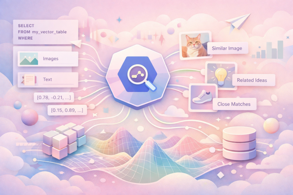
In this article, we will explore how Google quietly turned BigQuery into a full-fledged vector search and RAG platform. We will go from generating embeddings to semantic search using nothing but SQL. We will also discuss the trade-offs, showing exactly where this architecture shines and where (like high-load backends) it will fail miserably.
1. The Anatomy of Architectural Absurdity (Why Classic RAG is Broken)
To understand the beauty of native VECTOR_SEARCH in BigQuery, you need to realize how ugly the industry-standard RAG implementation actually is.
Imagine you have a table with 5 million products. The business wants a smart search so that when a user types “something warm for my feet,” the algorithm finds winter boots.
How the “Startup Playbook” does it:
- You write a Python script (or build an Airflow DAG) that runs a
SELECT *from BigQuery. You pay Google for data scanning and network egress. - The script sends these texts in batches to the OpenAI or Vertex AI API to generate embeddings (arrays of numbers).
- The script takes those vectors and makes
PUTrequests to Pinecone or Qdrant. - Congratulations, you now have two disconnected databases. BigQuery holds the business reality (prices, stock levels), and Pinecone holds vectors and product IDs.
Where the Nightmare Begins (Data Divergence):
A week later, a content manager updates 100,000 product descriptions in BigQuery. How does Pinecone know? It doesn’t. You now have to build a complex Change Data Capture (CDC) mechanism to track the delta, regenerate vectors, and push them to the third-party database. If Airflow crashes with an Out-of-Memory error (and it will), you get a “split brain.” A user finds a product via semantic search, but when the system tries to fetch the price, it returns NULL.
Data has gravity. Instead of building expensive, fragile pipelines to move data to the AI, it makes much more sense to bring the AI to the data.
2. The Setup: Digging a Tunnel to AI (Cloud Resource Connections)
BigQuery doesn’t store LLM models inside its compute slots. To generate embeddings, it needs to talk to Vertex AI. To do this, you set up a secure inter-service Connection.
Your infrastructure engineer does this once (ideally via Terraform, but clicking in the console works too):
- Create an External Connection of the
Cloud resourcetype in GCP. - GCP generates a unique service account for this connection.
- You go to IAM and grant this service account the
Vertex AI Userrole.
From a compliance perspective, this is a dream. Your data never leaves the Google Cloud perimeter. No API keys are passed in plain text, and no random startups are reading your corporate databases.
Now, we register the remote model directly in SQL. We’ll use a standard embedding model that understands dozens of languages.
SQL
CREATE OR REPLACE MODEL `my_project.analytics_dataset.embedding_model`
REMOTE WITH CONNECTION `eu.my_vertex_connection`
OPTIONS (
  ENDPOINT = 'text-multilingual-embedding-002'
);
That’s it. The neural network is now available as a standard SQL function.
3. Phase 1: Generating Embeddings (ML.GENERATE_EMBEDDING)
An embedding translates the meaning of text into the language of math. The AI takes your product description and turns it into an array (vector) of, say, 768 floating-point numbers. Concepts with similar meanings get arrays that are physically close to each other in a multi-dimensional space.
Let’s turn our raw catalog into a vector table with one elegant SQL query:
SQL
CREATE OR REPLACE TABLE `my_project.analytics_dataset.products_with_vectors` AS
SELECT
  product_id,
  product_name,
  category,
  price,
  description,
  -- All the magic happens right here
  ML.GENERATE_EMBEDDING(
    MODEL `my_project.analytics_dataset.embedding_model`,
    CONCAT(product_name, ' - ', description)
  ) AS embedding_data
FROM
  `my_project.analytics_dataset.raw_products`
WHERE
  description IS NOT NULL;
The FinOps Reality Check: The ML.GENERATE_EMBEDDING function returns a STRUCT containing the array and token statistics. You pay Vertex AI for the generation (usually fractions of a cent per 1,000 characters). Because BigQuery parallelizes this across thousands of nodes, generating vectors for a million rows takes minutes, not the hours your Python script would need.
4. Phase 2: Building the Vector Index (CREATE VECTOR INDEX)
If you try to search for nearest vectors using Brute Force, the database will compare your search query against every single vector in the table. This works for small datasets, but on a terabyte scale, it will eat your budget and take several minutes.
You need an Approximate Nearest Neighbor (ANN) algorithm. The main index type in BigQuery is IVF (Inverted File Index).
IVF clusters all vectors into “buckets” (lists) using the K-means method. When a search query arrives, the system doesn’t scan the whole database; it finds a few of the closest buckets and searches only inside them.
SQL
CREATE VECTOR INDEX product_semantic_index
ON `my_project.analytics_dataset.products_with_vectors`(embedding_data.ml_generate_embedding_result)
OPTIONS(
  index_type = 'IVF',
  distance_type = 'COSINE',
  ivf_options = '{"num_lists": 1000}'
);
The Parameters Explained:
distance_type = 'COSINE': Cosine distance is the gold standard for text. It measures the angle between vectors, ignoring their length. Meaning matters, not document size.num_lists: The number of clusters. More clusters mean faster searches, but a higher risk of missing the best match (lower Recall). Google recommends setting this to theSQRT(number_of_rows).
Index creation is asynchronous. And the best part? BigQuery automatically updates the index in the background when you insert or merge new rows. You don’t have to manually rebuild trees anymore.
5. Phase 3: Semantic Search (VECTOR_SEARCH)
Now our knowledge base is mathematically mapped and indexed. It’s time to write a query that will break the brain of any classic SQL analyst.
Suppose a customer searches for: “reliable rain protection for my laptop.” The word “protection” isn’t in the database; there’s only a “waterproof MacBook backpack.” A standard LIKE '%protection%' is completely useless here.
Enter VECTOR_SEARCH:
SQL
SELECT
  base.product_id,
  base.product_name,
  base.price,
  distance
FROM VECTOR_SEARCH(
  TABLE `my_project.analytics_dataset.products_with_vectors`,
  'embedding_data.ml_generate_embedding_result',
  (
    -- Generate a vector for the user's search query on the fly
    SELECT ML.GENERATE_EMBEDDING(
      MODEL `my_project.analytics_dataset.embedding_model`,
      'reliable rain protection for my laptop'
    ) AS query_embedding
  ),
  top_k => 5,
  distance_type => 'COSINE'
)
ORDER BY distance ASC;
BigQuery will return the top 5 semantic matches. You get instant access to the product ID and its current price without needing to JOIN another database, because the search happens directly on your primary table.
6. Phase 4: Closing the RAG Loop in SQL (LLM Integration)
If we are building a customer support Q&A bot, just finding paragraphs of text isn’t enough. We need to feed them to an LLM to generate a human-friendly answer.
Once again, data doesn’t go anywhere. We call Gemini Pro right inside SQL using ML.GENERATE_TEXT.
Here is a complete RAG pipeline in one single SQL query:
SQL
WITH SemanticMatches AS (
  SELECT
    base.description AS chunk_text
  FROM VECTOR_SEARCH(
    TABLE `my_project.analytics_dataset.support_docs_vectors`,
    'embedding',
    (SELECT ML.GENERATE_EMBEDDING(MODEL `my_project.embedding_model`, 'How do I reset the admin password?')),
    top_k => 3
  )
)
SELECT
  ML.GENERATE_TEXT(
    MODEL `my_project.analytics_dataset.gemini_pro`,
    CONCAT(
      'You are a technical assistant. Answer the user using ONLY the following context. If the answer is not there, say "I don\'t know."\n\n',
      'Context:\n',
      (SELECT STRING_AGG(chunk_text, '\n---\n') FROM SemanticMatches),
      '\n\nQuestion: How do I reset the admin password?'
    ),
    STRUCT(0.1 AS temperature, 500 AS max_output_tokens)
  ) AS llm_response;
From an architectural standpoint, this is phenomenal. You just built a full Retrieval-Augmented Generation pipeline writing exactly zero lines of Python and deploying zero microservices.
7. Architectural Trade-offs (The Harsh Reality)
Like any seasoned R&D engineer, you know there are no silver bullets. Native vector search in BigQuery has strict limitations. Ignoring them will guarantee your project’s spectacular failure.
- Limitation 1: Latency (Highload is a No-Go): BigQuery is an OLAP database built for chewing through petabytes of data, not for millisecond responses. A
VECTOR_SEARCHquery takes 1 to 4 seconds. If you are building a high-load Go backend that processes 150,000 RPS and needs to deliver search autocomplete to a mobile app in 50 milliseconds, BigQuery is absolutely not for you. For real-time, user-facing production traffic, you still need a caching layer or a specialized OLTP database (like PostgreSQL withpgvectoron AlloyDB). - Limitation 2: FinOps Disasters: Pinecone charges for server uptime and RAM. BigQuery charges for data scanned. If your index is poorly built or you use a low
num_lists, BigQuery might fall back to a Full Table Scan. Vector columns are heavy. A full scan of a terabyte vector table will cost you a small fortune per query. Without proper Quotas and indexing, semantic search will eat your cloud budget over the weekend. - Limitation 3: Pre-filtering Mechanics: Modern vector databases can filter during the search (e.g., “find semantic matches, but only where
price < 100“). BigQuery finds thetop_kclosest vectors first, and then applies SQL filters. If you ask for 10 items and 9 of them are out of stock, the user only sees 1 result. You have to artificially inflate yourtop_kparameter (e.g., fetch 1,000 and filter), which increases compute costs.
8. Where This Works Perfectly
Despite OLTP limitations, this architecture is an absolute killer for Data Engineering, internal analytics, and background processes.
- Data Quality & Fuzzy Matching (Deduplicating Chaos): Your CRM records the same company as “John Doe Inc.”, “J. Doe Incorporated”, and a typo “Jphn Doe Inc”. Standard SQL and regex will never figure this out. Vector search inside BigQuery turns names into embeddings and finds hidden clusters. You can automatically merge duplicate contractors with 98% confidence.
- Log Clustering for Observability: When infrastructure crashes, it generates millions of logs. For a classic
GROUP BY,Connection timeout on 10.1.1.1andTimeout error on 192.168.0.5are two different strings. By embedding error texts, a DataOps engineer can useVECTOR_SEARCHto collapse millions of logs into 5 meaningful clusters, drastically cutting down Root Cause Analysis time. - Asynchronous Ticket Classification: Customer support gets 10,000 tickets a day. Instead of exporting them to Python, you run a Scheduled Query in BQ every 15 minutes. It generates vectors for new tickets, finds semantically similar historical solutions (RAG), and drafts a response for the human operator. A 3-second latency here doesn’t matter, but the infrastructure savings are huge.
Conclusion
The data industry moves in cycles. First, we exported data out of databases into specialized engines to do complex math. Now, database compute power has grown so much that the math is coming back to the data.
BigQuery Vector Search is a prime example of Data Gravity. Killing ETL pipelines, getting rid of a zoo of third-party vector databases, maintaining centralized IAM security, and building RAG with plain SQL—this changes the game for data engineers.
It is not a magic pill for mobile real-time search. But for the vast majority of corporate semantic analysis, data normalization, and LLM integration tasks, GCP’s native architecture saves months of development and tens of thousands of dollars in infrastructure budget. Stop building duct-tape architectures where a simple SELECT will do.
We build, migrate, and optimize cloud data pipelines on Google Cloud Platform. From BigQuery query optimization to custom ingestion architectures, explore our Data Engineering on GCP services.